Research · Jul 19, 2026
Inside a Tiny Transformer
A reproducible mechanistic interpretability study of how tiny transformers learn modular addition, develop Fourier structure, and distribute causal computation across nearly the entire model.
Introduction
What does “understanding” look like inside a neural network? To study that question at a scale where every weight can be inspected, we trained a deliberately tiny transformer — two layers, four attention heads, a 128-dimensional residual stream, 512-neuron MLPs, no LayerNorm, 419,840 parameters in all — on a single task: adding two numbers on a 97-hour clock, a + b mod 97.
There are 9,409 possible input pairs. The model saw 40% of them during training and was tested on the remaining 60%. We ran the experiment five times from different random seeds and then took the trained networks apart with the standard tools of mechanistic interpretability: Fourier analysis, direct logit attribution, activation patching, path patching, and automated circuit discovery.
What the model learned
All five runs ended accurate: final test accuracy ranged from 98.88% to 100.00% (mean 99.4%). More interesting than that the model learned is what it learned. Rather than memorizing a lookup table, the network invented trigonometry: it represents each number as a set of rotations at a few chosen frequencies, adds angles to add numbers, and reads the answer back out — the “Fourier multiplication” algorithm first described in one-layer models by Nanda et al. (2023), reproduced here in two-layer models in four of five runs.
Grokking
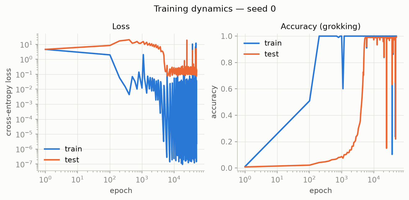
The path to that algorithm was anything but smooth. Every run memorized its training set within 200 epochs — and then sat at near-zero test accuracy for thousands of epochs before suddenly generalizing, at epoch 3,300 to 5,900 depending on the seed. That is a 16–30× gap between memorization and understanding, the signature of grokking.
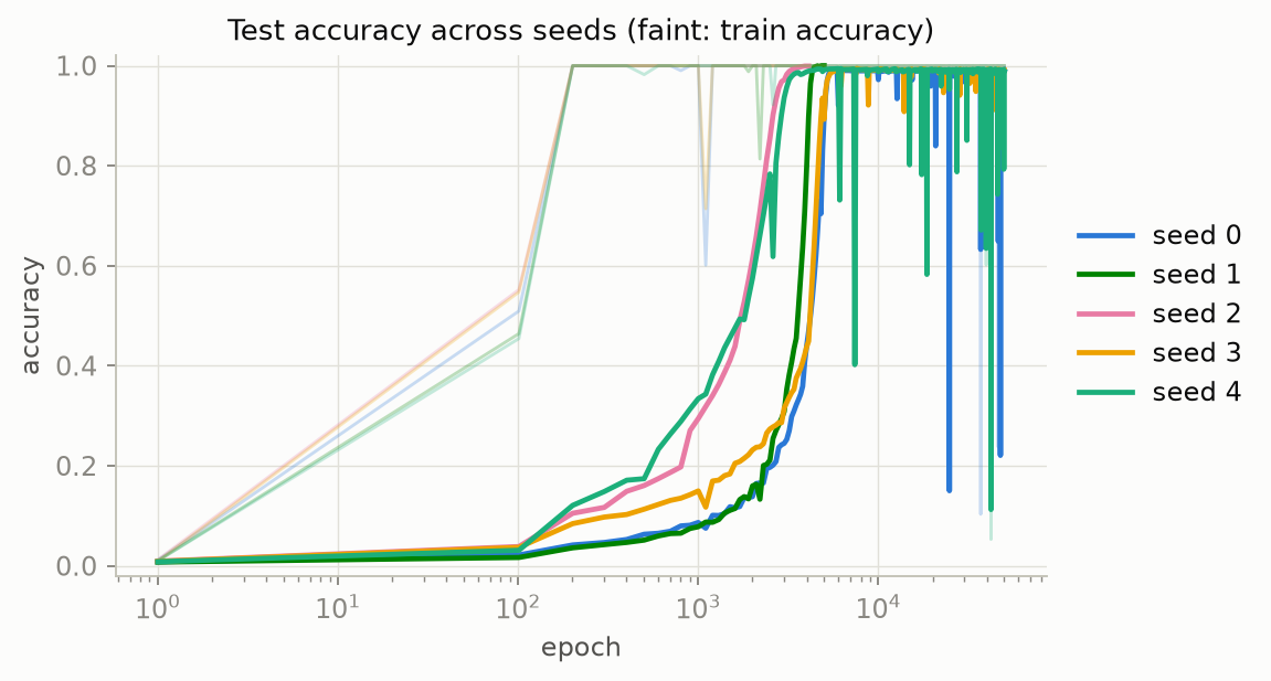
Training was also punctuated by “slingshots” — transient collapse-and-recovery events in which train accuracy fell below 90% after having reached 99%. Four of the five runs show them; the deepest collapse fell to 5.3% train accuracy before recovering within roughly a thousand epochs.
Fourier structure
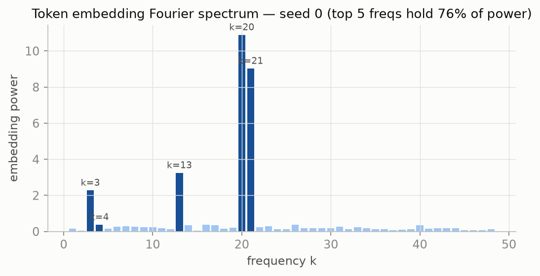
The clearest fingerprint of the invented algorithm sits in the learned number embeddings. Decomposed into waves, 76.0–87.3% of their (non-constant) power concentrates in just five of 48 possible frequencies — a flat spectrum would put 10.4% there. Every seed shows this sparsity, but each picks its own, largely disjoint frequency set: seed 0 chose {3, 4, 13, 20, 21}, seed 2 chose {10, 12, 14, 35, 45}. The algorithm replicates; its parameters do not.
The output side tells the same story. Projecting the model’s centered logits onto the rotation formula cos/sin(2πk(a+b−c)/97) over each seed’s key frequencies explains R² = 0.877, 0.950, 0.851, 0.760, and 0.562 of the variance for seeds 0–4 (mean 0.800 ± 0.150). Four of five runs fit the formula well (0.76–0.95); seed 4 is the exception we return to below.
Causal interventions
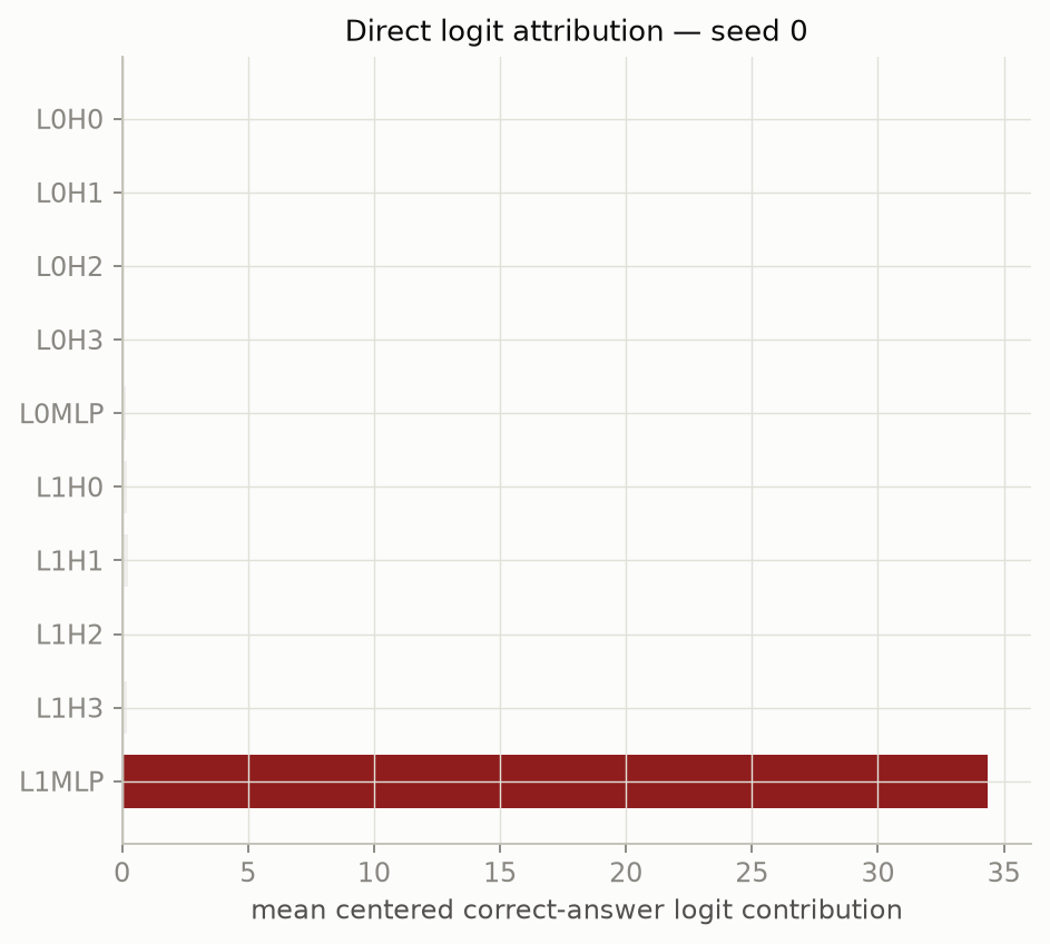
Correlational evidence is not enough: a component can look important without being causally necessary, and vice versa. The cleanest illustration is direct logit attribution, which measures each component’s direct write onto the correct answer. By that measure the layer-1 MLP dominates and layer-0 components write almost nothing — yet ablating layer 0 is devastating. Layer 0 acts entirely through layer 1, and purely correlational rankings miss it.
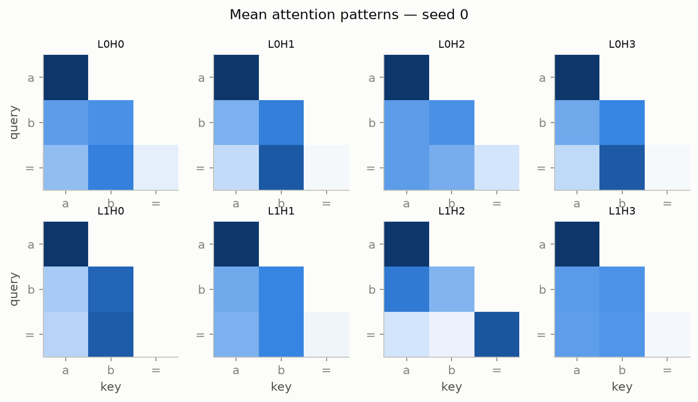
What does attention contribute? Not arithmetic — routing. In the final row of every head’s attention map, the “=” position that must produce the answer attends to the two operand positions, moving a and b into place for the MLPs to combine.
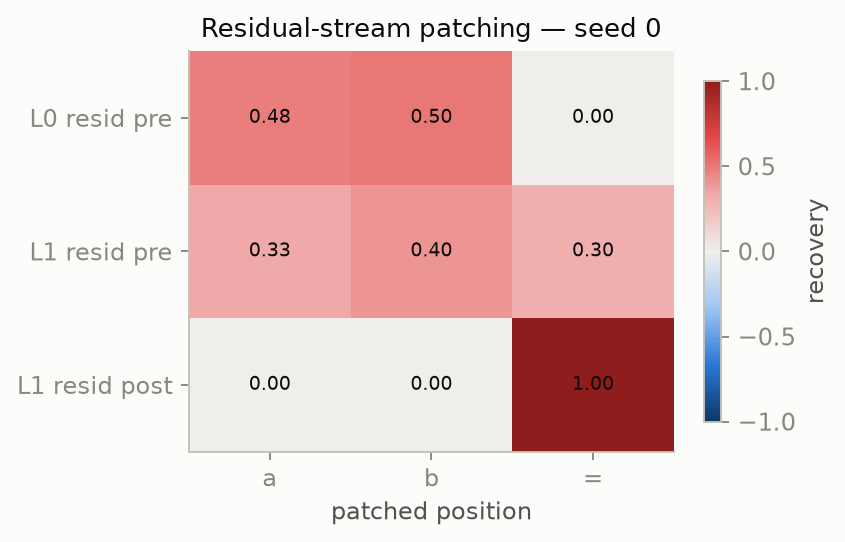
Patching the residual stream maps the computation in space: answer information sits at the operand positions entering layer 0 (recovery 0.48 / 0.50), spreads by layer 1, and lives entirely at the “=” position at the end (1.00).
The compact-circuit hypothesis
A central hope of mechanistic interpretability is that trained networks decompose into compact circuits: small subsets of components that carry a behavior on their own. We tested that hypothesis directly with greedy backward elimination — remove components one at a time, always keeping the subset that best preserves accuracy under mean ablation — and asked what survives at a 95% faithfulness bar.
Negative result: distributed computation
Nothing compact survives. At the 95% bar, the search retained the entire model — all 10 components — in four of five seeds, and 9 of 10 in the fifth. This is a negative result, and we report it as one: the threshold sets are not discovered circuits, and mean-ablating them collapses test accuracy to 0.87–1.19%, indistinguishable from chance (1.03%).
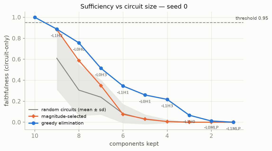
The decay is structured, not random: greedy selection beats both random same-size sets and activation-magnitude selection at every size of two or more, in every seed. For seed 0 at size 8, greedy retains 0.756 versus 0.306 ± 0.245 for random and 0.587 for magnitude; at size 4 the gap is 0.218 versus 0.008 and 0.006. Importance is graded and structured — each head carries a share of the same signals — but it is not modular.
The same holds one level down: there is no neuron-level sparsity. Recovering 90% of performance requires 410–425 of 512 layer-0 MLP neurons and 274–386 of 512 layer-1 MLP neurons — 54–83% of each MLP.
Cross-seed findings
Five runs, one algorithm, five personalities. Grokking, sparse Fourier embeddings, and distributed computation replicate in every seed — while the key frequencies, the timing of generalization, and the quality of the rotation-formula fit are seed-specific.
| Seed | Test acc. | Generalizes at | Top-5 power | Logit R² | Key frequencies |
|---|---|---|---|---|---|
| 0 | 99.19% | 5,700 | 76.0% | 0.877 | 3, 4, 13, 20, 21 |
| 1 | 100.00% | 4,300 | 83.0% | 0.950 | 10, 13, 20, 35, 42 |
| 2 | 99.91% | 3,300 | 87.3% | 0.851 | 10, 12, 14, 35, 45 |
| 3 | 99.10% | 5,900 | 79.2% | 0.760 | 3, 8, 10, 13, 42 |
| 4 | 98.88% | 4,200 | 82.0% | 0.562 | 29, 31, 34, 35, 48 |
Seed 4 is the honest asterisk: its accuracy is normal (98.88%) and its embeddings are sparse, but the rotation formula explains only R² = 0.562 of its logit variance — and stays at 0.562 when the frequency set is widened to the top 8, 12, or 20 embedding frequencies. Whatever computes the remaining structure in seed 4 is uncharacterized.
Limitations
- Training-duration confound: seeds stopped between 4,101 and 50,000 epochs under one uniform stopping rule; cross-seed differences partly reflect training time. A matched-schedule control configuration ships with the repository.
- Seed 4 fits the Fourier-interference model poorly (R² 0.562, invariant to widening the frequency set); its residual structure is uncharacterized.
- No compact head-level circuit exists at the 95% faithfulness bar (a negative result), and there is no neuron-level sparsity either (54–83% of neurons needed).
- Mean ablation defines every counterfactual; other ablation choices could shift circuit boundaries.
- Greedy backward elimination does not certify global minimality; neuron refinement is prefix selection, not joint search.
- All seeds share one train/test split (deliberate, for circuit comparability).
- Five seeds and 20 baseline resamples support descriptive statistics only; no significance tests are claimed.
Explore the full visualization
The full study is available as an interactive experience: scroll through the story of the network — the 97-position clock, the grokking moment, the Fourier spectra, and the causal interventions — or open the Research Explorer to examine every underlying chart and table yourself.
Prefer the raw data? The Research Explorer exposes every chart, ranking, and definition behind the story.
GitHub and technical report
The repository is private at the time of writing; these links require collaborator access until it is made public.